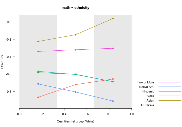
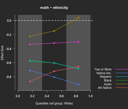
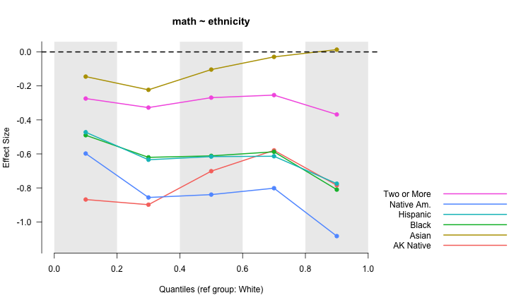
esvis: An R package for effect size visualizations

Daniel Anderson

Univeristy of Oregon

Background

Effect sizes quantify the magnitude of effects

  • Generally defined by standardized mean differences
    • Cohen's d
    • Hedges' g
  • Particularly in non-experimental settings, interest may lie at other locations of the scale
    • Educational achievement gaps between student subgroups at "proficiency" cut points
  • Depending on the shape of each distribution, magnitude of group differences may depend upon scale location

Cohen's d & Hedges' g


\[d = \frac{\bar{X}_{foc} - \bar{X}_{ref}} {\sqrt{\frac{(n_{foc} - 1)Var_{foc} + (n_{ref} - 1)Var_{ref}} {n_{foc} + n_{ref} - 2}}}\]

\[g = d\Big(1 - \frac{3}{4(n_{foc} + n_{ref}) - 9}\Big)\]

Percentage above the cut effect sizes

Percentage Above the Cut

\[d^{pac} = PAC_{ref} - PAC_{foc}\]

  • Highly dependent on scale location

Transformed Percentage Above the Cut

\[d^{tpac} = \Phi^{-1}(PAC_{ref}) - \Phi^{-1}(PAC_{foc})\]

  • Assumes both distributions are normally distributed with equal variance

Probability-Probability Plots

plot of chunk ecdf1

plot of chunk pp_plot1

Area Under the PP Curve

plot of chunk auc

Putting AUC in SD units

Ho and colleagues

\[V = \sqrt{2}\Phi^{-1}(AUC)\]

  • Scale invariant
  • Assumes respective normality
    • Normal with respect to each other under a shared transformation


  • AUC and V make fewer assumptions about the data, but are nonetheless summary measures.
  • May miss nuances in the data that can be picked up by visualizations - particularly if the magnitude of the effect depends on scale location.

Implementation in esvis

R package actively in development

  • Install using the devtools package
install.packages("devtools")
library(devtools) 
install_github("DJAnderson07/esvis")
  • Release to CRAN planned for summer
  • Has many useful features currently


See current development at

https://github.com/DJAnderson07/esvis

esvis

Example data

I have stored a dataset in an object called d. Below are the first six rows of these data.

##         sid cohort     sped  ethnicity frl     ell season reading math
## 2873 332347      1 Non-Sped   Hispanic FRL  Active Spring     167  192
## 162  400047      1 Non-Sped Native Am. FRL Non-ELL Spring     191  191
## 355  400047      1 Non-Sped Native Am. FRL Non-ELL   Fall     183  182
## 387  400047      1 Non-Sped Native Am. FRL Non-ELL Winter     178  179
## 230  400277      1 Non-Sped Native Am. FRL Non-ELL Winter     199  197
## 648  400277      1 Non-Sped Native Am. FRL Non-ELL   Fall     203  196

Standard argument structure

  • All functions in esvis take a common argument structure, as follows
fun_name(outcome ~ group, data, additional_optional_args)

PP Plots

  • Examine math differences by free or reduced lunch status
pp_plot(math ~ frl, d)
  • Notice shading by default when only two groups are compared.
  • AUC and V annotated to the plot, by default
  • Plot is fully customizable with calls to base plotting functions (e.g., main, col, etc.)

plot of chunk frl_pp_plot_eval

More than one group?

  • Highest performing group selected by default
pp_plot(reading ~ ethnicity, d)

plot of chunk pp_plot_eth

Investigating ELL differences

  • Three groups: Non, Active, Monitor
  • Same syntax for estimates

Default output

coh_d(reading ~ ell, d)
##   ref_group foc_group    estimate
## 1   Monitor   Non-ELL  0.05421767
## 2   Monitor    Active  0.70109139
## 3   Non-ELL    Active  0.95679846
## 4    Active   Non-ELL -0.95679846
## 5    Active   Monitor -0.70109139
## 6   Non-ELL   Monitor -0.05421767

Or choose a reference group

auc(reading ~ ell, d, 
        ref_group = "Non-ELL")
##   ref_group foc_group  estimate
## 3   Non-ELL    Active 0.7552992
## 6   Non-ELL   Monitor 0.4965789

Visualization provides more nuance

pp_plot(reading ~ ell, d, ref_group = "Non-ELL")

plot of chunk pp_plot_ell

ECDFs

  • Produced equivalently
ecdf_plot(reading ~ ell, d)

plot of chunk ecdf_ell1

Cut-point?

ecdf_plot(reading ~ ell, d, ref_cut = c(190, 200, 207))

plot of chunk ecdf_ell2

Add horizontal reference lines

ecdf_plot(reading ~ ell, d, ref_cut = c(190, 200, 207), hor_ref = TRUE)

plot of chunk ecdf_ell3

Binned ES Plot

  • Split each distribution into arbitrary (even) quantile bins
  • Calculate mean difference within each bin
  • Divide by overall pooled standard deviation

\[d_{[i]} = \frac{\bar{X}_{foc_{[i]}} - \bar{X}_{ref_{[i]}}} {\sqrt{\frac{(n_{foc} - 1)Var_{foc} + (n_{ref} - 1)Var_{ref}} {n_{foc} + n_{ref} - 2}}}\]

  • In this case, essentially equivalent to Cohen's d, except that there are multiple mean differences (one for each bin)

Ethnicity differences

binned_plot(math ~ ethnicity, d)

plot of chunk binned_es_plot_eth1

Change binning

Quintile binning

binned_plot(math ~ ethnicity, d, qtiles = seq(0, 1, .2))

plot of chunk binned_es_plot_eth2

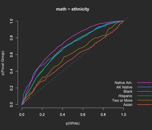
coh_d(math ~ ethnicity, d)
##      ref_group   foc_group    estimate
## 1        White       Asian  0.10689571
## 2        White Two or More  0.30281232
## 3        White    Hispanic  1.03147010
## 4        White       Black  0.72127040
## 5        White   AK Native  0.76483392
## 6        White  Native Am.  0.84185433
## 7        Asian Two or More  0.07471180
## 8        Asian    Hispanic  0.72590767
## 9        Asian       Black  0.39210777
## 10       Asian   AK Native  0.29878405
## 11       Asian  Native Am.  0.39455423
## 12 Two or More    Hispanic  0.40811606
## 13 Two or More       Black  0.21475724
## 14 Two or More   AK Native  0.16297587
## 15 Two or More  Native Am.  0.24174797
## 16    Hispanic       Black  0.02423883
## 17    Hispanic   AK Native  0.25579261
## 18    Hispanic  Native Am.  0.30800593
## 19       Black   AK Native  0.12256685
## 20       Black  Native Am.  0.15962973
## 21   AK Native  Native Am.  0.01700166
## 22  Native Am.   AK Native -0.01700166
## 23  Native Am.       Black -0.15962973
## 24  Native Am.    Hispanic -0.30800593
## 25  Native Am. Two or More -0.24174797
## 26  Native Am.       Asian -0.39455423
## 27  Native Am.       White -0.84185433
## 28   AK Native       Black -0.12256685
## 29   AK Native    Hispanic -0.25579261
## 30   AK Native Two or More -0.16297587
## 31   AK Native       Asian -0.29878405
## 32   AK Native       White -0.76483392
## 33       Black    Hispanic -0.02423883
## 34       Black Two or More -0.21475724
## 35       Black       Asian -0.39210777
## 36       Black       White -0.72127040
## 37    Hispanic Two or More -0.40811606
## 38    Hispanic       Asian -0.72590767
## 39    Hispanic       White -1.03147010
## 40 Two or More       Asian -0.07471180
## 41 Two or More       White -0.30281232
## 42       Asian       White -0.10689571

Change reference group

binned_plot(math ~ ethnicity, d, ref_group = "Black", qtiles = seq(0, 1, .2))

plot of chunk binned_es_plot_eth3

Theme dark

pp_plot(math ~ ethnicity, d, 
    theme = "dark")

plot of chunk theme_standard

binned_plot(math ~ ethnicity, d, 
    theme = "dark")

plot of chunk theme_dark

Estimation

esvis will also calculate a number of effect sizes using the same argument structure, including:

  • Cohen's d
  • Hedges' g
  • AUC
  • V
  • PAC with any set of cut scores
  • TPAC with one cut score (currently)

By default, effect sizes are produced for all possible pairwise comparisons, but reference groups can be selected as well.

Summary and future developments

  • Visualizing group differences across the full scale, or at particular points of the scale, is important for interpretation and communication.
  • esvis provides a simple interface to produce powerful visualizations

Future development

  • Interactions with : and via panel plotting
  • Including uncertainty
  • Others?

Thanks!