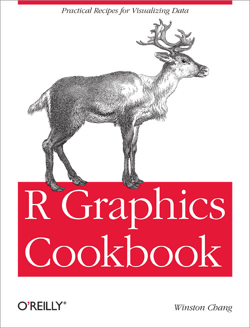
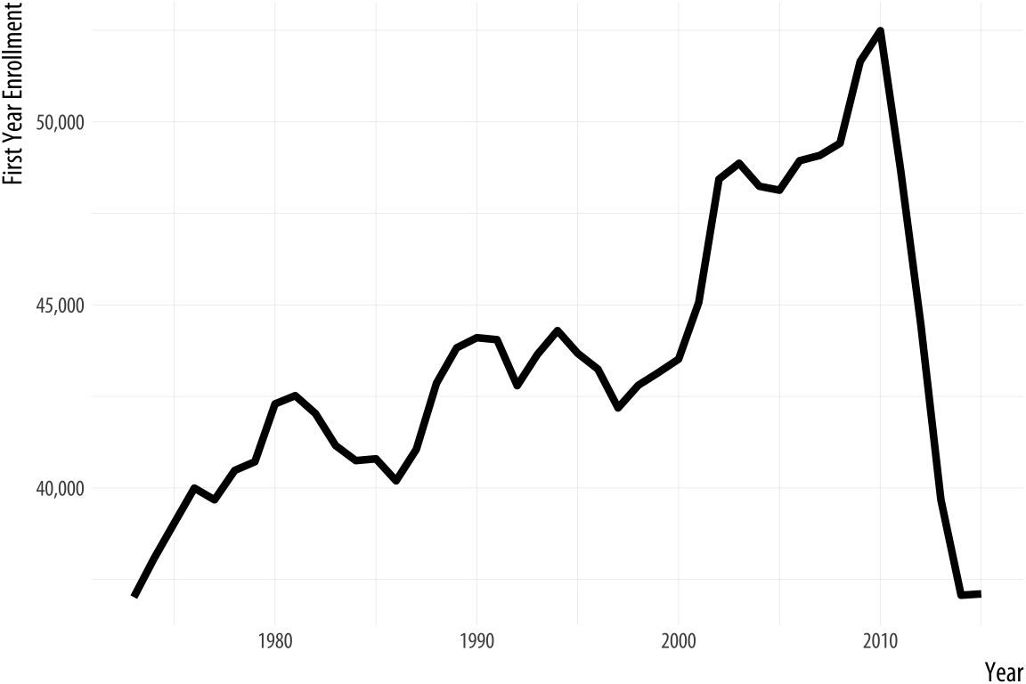
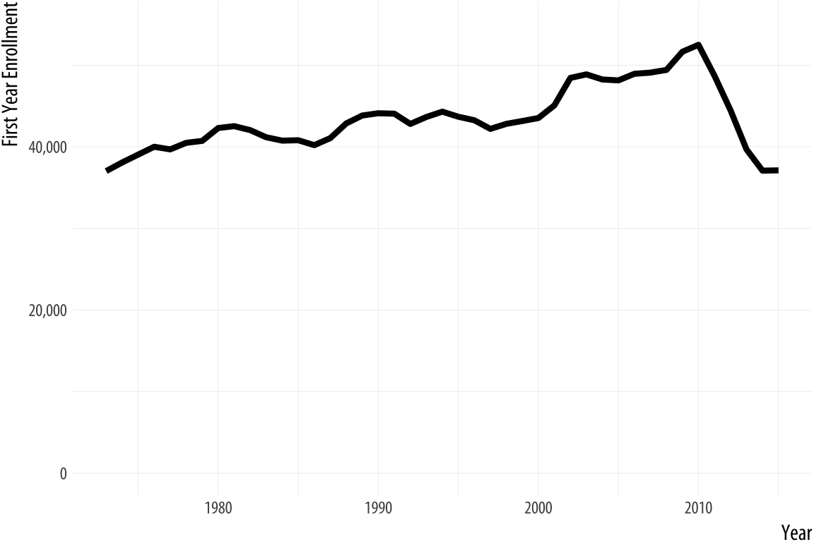
class: center, middle, inverse, title-slide # Some data viz advice ### Daniel Anderson ### Monday, May 13, 2021 --- layout: true <script> feather.replace() </script> <div class="slides-footer"> <span> <a class = "footer-icon-link" href = "https://github.com/datalorax/cos-dataviz/raw/main/anderson-cos-dataviz.pdf"> <i class = "footer-icon" data-feather="download"></i> </a> <a class = "footer-icon-link" href = "https://datalorax.github.io/cos-dataviz"> <i class = "footer-icon" data-feather="link"></i> </a> <a class = "footer-icon-link" href = "https://github.com/datalorax/cos-dataviz"> <i class = "footer-icon" data-feather="github"></i> </a> </span> </div> --- # whoami .pull-left[ * Research Assistant Professor: Behavioral Research and Teaching * Dad (two daughters: 8 and 6) * Pronouns: he/him/his * Primary areas of interest: 💗💗R💗💗, computational research, systemic inequities in educational systems and variance between educational institutions ] .pull-right[  </div> ] --- # Resources (free) .pull-left[ [Healy](http://socviz.co) <div> <img src = http://socviz.co/assets/dv-cover-pupress.jpg height = 400> </div> ] .pull-right[ [Wilke](https://serialmentor.com/dataviz/) <div> <img src = https://external-content.duckduckgo.com/iu/?u=http%3A%2F%2Febook3000.com%2Fupimg%2Fallimg%2F190330%2F0153540.jpg&f=1&nofb=1 height = 400> </div> ] --- # Other Resources * My classes! * Sequence + EDLD 651: Introductory Educational Data Science (EDS) + EDLD 652: [Data Visualization for EDS](https://dataviz-2021.netlify.app/) + EDLD 653: [Functional Programming for EDS](https://fp-2021.netlify.app/) + EDLD 654: [Machine Learning for EDS](https://uo-datasci-specialization.github.io/c4-ml-fall-2020/index) + Capstone --- # Where to start? * I *really* recommend moving to R as quickly as possible, if you haven't already -- .center[ [R for Data Science](http://r4ds.had.co.nz) <div> <img src = img/r4ds.png height = 350> </div> ] --- # ggplot2! .pull-left[ https://r-graphics.org  ] .pull-right[ Third edition [in progress](https://ggplot2-book.org)!  ] --- # Last note before we really start * These slides were produced with R * See the source code [here]() * The focus of this particular talk is not on the code itself --- class: middle center # Different ways of encoding data <!-- --> .footnote[Code from [Wilke](https://clauswilke.com/dataviz/)] --- # Other elements to consider * Text + How is the text displayed (e.g., font, face, location)? + What is the purpose of the text? -- * Transparency + Are there overlapping pieces? + Can transparency help? --- # Encoding data? How might we encode these data into a display? | Month | Day | Location | Temperature | |:-----:|:---:|:-------------| ------------| | Jan | 1 | Chicago | 25.6 | | Jan | 1 | San Diego | 55.2 | | Jan | 1 | Houston | 53.9 | | Jan | 1 | Death Valley | 51.0 | | Jan | 2 | Chicago | 25.5 | | Jan | 2 | San Diego | 55.3 | | Jan | 2 | Houston | 53.8 | | Jan | 2 | Death Valley | 51.2 | | Jan | 3 | Chicago | 25.3 | .footnote[Example from [Wilke](https://clauswilke.com/dataviz/)] --- # One option <!-- --> .footnote[Example from [Wilke](https://clauswilke.com/dataviz/)] --- class: middle center # Alternative representation <!-- --> .footnote[Example from [Wilke](https://clauswilke.com/dataviz/)] --- # Comparison * Both represent three scales + Two position scales (x/y axis) + One color scale (categorical for the first, continuous for the second) --- background-image:url(http://socviz.co/dataviz-pdfl_files/figure-html4/ch-01-multichannel-1.png) background-size:contain # More scales are possible But can become lost without high structure in the data .footnote[Example from [Healy](https://socviz.co/)] --- class: inverse-blue middle # Thinking more about color --- # Three fundamental uses 1. Distinguish groups from each other 1. Represent data values 1. Highlight --- # Discrete items Often no intrinsic order -- ### Qualitative color scale * Finite number of colors + Chosen to maximize distinctness, while also being *equivalent* + Equivalent - No color should stand out - No impression of order --- # Examples .footnote[See more about the Okabe Ito palette origins [here](http://jfly.iam.u-tokyo.ac.jp/color/)] <!-- --> --- # Sequential scale examples <!-- --> --- # Diverging palettes <!-- --> --- # Earth palette Applied example: Percentage of people coded "white" in California according to the 2010 decennial census. <!-- --> --- # Common problems ### Too many colors More than 5-ish generally becomes difficult to track <!-- --> .footnote[Data from [Wilke](https://clauswilke.com/dataviz/)] --- # Use labels still too many... <!-- --> .footnote[Data from [Wilke](https://clauswilke.com/dataviz/)] --- # Better Get a subset <!-- --> .footnote[Data from [Wilke](https://clauswilke.com/dataviz/)] --- # Best (but could still be improved) <!-- --> .footnote[Data from [Wilke](https://clauswilke.com/dataviz/)] --- # Last few note on palettes * Do some research, find what you like **and** what tends to work well * Check for colorblindness (many options, but consider [here](https://www.color-blindness.com/coblis-color-blindness-simulator/)) * Look into http://colorbrewer2.org/ --- class: inverse-blue middle # Visualizing Uncertainty --- # The primary problem * When we see a point on a plot, we interpret it as **THE** value. <!-- --> --- # Some secondary problem * We're not great at understanding probabilities * We regularly round probabilities to 100% or 0% * As probabilities move to the tails, we're generally worse --- # How do we typically communicate uncertainty? * Error bars <!-- --> --- # Thinking about uncertainty Uncertainty means exactly what it sounds like - we are not 100% sure. * We are nearly always uncertain of future events (forecasting) * We can also be uncertain about past events + I saw a parked car at 8 AM, but the next time I looked at 2PM it was gone. What time did it leave? -- ### Quantifying uncertainty * We quantify our uncertainty mathematically using probability * Framing probabilities as frequencies is generally more intuitive --- class: bottom background-image:url("https://serialmentor.com/dataviz/visualizing_uncertainty_files/figure-html/probability-waffle-1.png") background-size:contain # Framing a single uncertainty .footnote[Example from [Wilke](https://clauswilke.com/dataviz/)] --- # Non-discrete probabilities Blue party has 1% advantage w/ margin of error of 1.76 points ### Who will win? -- <!-- --> .footnote[Code taken from [Wilke](https://clauswilke.com/dataviz/)] --- # Descretized version <!-- --> --- class: inverse-red middle # Point estimates A few alternatives to error bars --- # Multiple error bars <!-- --> --- # Density stripes <!-- --> --- # Actual densities <!-- --> --- class: inverse-red middle # HOPs ### Hypothetical Outcome Plots (and related plots) --- # Standard regression plot <!-- --> --- # Alternative <!-- --> --- # HOPs Hops animate the process, so you can't settle on one "truth"  --- # Last few notes on uncertainty * Do try to communicate uncertainty whenever possible * I'd highly recommend watching [this](https://youtu.be/E1kSnWvqCw0) talk by Matthew Kay on the topic --- class: inverse-blue middle # Data ink ratio --- # What is it? -- > ### Above all else, show the data <br> \-Edward Tufte -- * Data-Ink Ratio = Ink devoted to the data / total ink used to produce the figure -- * Common goal: Maximize the data-ink ratio --- # Example  -- * First thought might be... Cool! --- background-image:url(https://theamericanreligion.files.wordpress.com/2012/10/lee-corso-sucks.jpeg?w=660) background-size:cover --- # Minimize cognitive load * Empirically, Tufte's plot was .bolder[the most difficult] for viewers to interpret. -- * Visual cues (labels, gridlines) reduce the data-ink ratio, but can also reduce cognitive load. --- # An example ### Which do you prefer? .pull-left[ <!-- --> ] .pull-right[ <!-- --> ] .footnote[Code/example taken from [Wilke](https://clauswilke.com/dataviz/)] --- # Advice from Wilke > Whenever possible, **visualize your data with solid, colored shapes** rather than with lines that outline those shapes. Solid shapes are more easily perceived, are less likely to create visual artifacts or optical illusions, and do more immediately convey amounts than do outlines. .gray[emphasis added] --- # Another example .pull-left[ <!-- --> ] .pull-right[ <!-- --> ] .footnote[Code/example taken from [Wilke](https://clauswilke.com/dataviz/)] --- class: center middle <!-- --> .footnote[Code/example taken from [Wilke](https://clauswilke.com/dataviz/)] --- # Labels in place of legends Prior slide is a great example of when annotations can be used in place of a legend to * reduce cognitive load * increase clarity * increase beauty * maximize the figure size --- class: inverse-red middle # Practical advice so far --- class: inverse-red middle ## Include uncertainty wherever possible <br> -- ## Avoid line drawings <br> -- ## Maximize the data-ink ratio within reason (but preference reduction of cognitive load) --- class: inverse-red middle ## Use color to your advantage (and think critically about the palettes you choose) <br> -- ## Consider plot annotations over legends --- class: inverse-red middle # Dealing with grouped data ### Quick empirical example --- # Titanic data ``` ## # A tibble: 1,313 x 5 ## name class age sex survived ## <chr> <chr> <dbl> <chr> <int> ## 1 Allen, Miss Elisabeth Walton 1st 29 female 1 ## 2 Allison, Miss Helen Loraine 1st 2 female 0 ## 3 Allison, Mr Hudson Joshua Creighton 1st 30 male 0 ## 4 Allison, Mrs Hudson JC (Bessie Waldo Daniels) 1st 25 female 0 ## 5 Allison, Master Hudson Trevor 1st 0.92 male 1 ## 6 Anderson, Mr Harry 1st 47 male 1 ## # … with 1,307 more rows ``` --- # Boxplots <!-- --> --- # Jittered point plots <!-- --> --- # Sina plot <!-- --> --- # Stacked histogram <!-- --> -- .realbig[🤨] --- # Dodged <!-- --> --- # Better <!-- --> --- # Overlapping densities <!-- --> --- # Ridgeline densities <!-- --> --- class: inverse-red middle # Visualizing amounts ### How much does college cost? --- # Tuition data ``` ## # A tibble: 6 x 13 ## State `2004-05` `2005-06` `2006-07` `2007-08` `2008-09` `2009-10` ## <chr> <dbl> <dbl> <dbl> <dbl> <dbl> <dbl> ## 1 Alabama 5682.838 5840.550 5753.496 6008.169 6475.092 7188.954 ## 2 Alaska 4328.281 4632.623 4918.501 5069.822 5075.482 5454.607 ## 3 Arizona 5138.495 5415.516 5481.419 5681.638 6058.464 7263.204 ## 4 Arkansas 5772.302 6082.379 6231.977 6414.900 6416.503 6627.092 ## 5 California 5285.921 5527.881 5334.826 5672.472 5897.888 7258.771 ## 6 Colorado 4703.777 5406.967 5596.348 6227.002 6284.137 6948.473 ## # … with 6 more variables: 2010-11 <dbl>, 2011-12 <dbl>, 2012-13 <dbl>, ## # 2013-14 <dbl>, 2014-15 <dbl>, 2015-16 <dbl> ``` --- # By state: 2015-16 <!-- --> -- .realbig[🤮🤮🤮] --- # Two puke emoji version .pls[ .realbig[🤮🤮] ] .prb[ <!-- --> ] --- # One puke emoji version .pls[ .realbig[🤮] ] .prb[ <!-- --> ] --- # Kinda smiley version .pls[ .realbig[😏] ] .prb[ <!-- --> ] --- # Highlight a state .pls[ .realbig[🙂] ] .prb[ <!-- --> ] --- # Not always good to sort <!-- --> --- # Much better <!-- --> --- # Heatmap <!-- --> --- # Better heatmap <!-- --> --- # Even better? <!-- --> --- # Or maybe this one? <!-- --> --- background-image: url("img/heatmap.png") class: inverse-blue background-size:contain --- # Quick aside * Think about the data you have * Given that these are state-level data, they have a geographic component --- background-image: url("img/states-heatmap.png") class: inverse bottom background-size:contain --- class: inverse-blue center middle # Some things to avoid --- # Line drawings ### As discussed earlier .pull-left[ ### 😫 <!-- --> ] .pull-right[ ### Change the fill <!-- --> ] --- # Much worse ### Unnecessary 3D .pull-left[  ] .pull-right[  ] --- # Much worse ### Unnecessary 3D .pull-left[  ] .pull-right[  ] --- # Horrid example ### Used relatively regularly  --- # Pie charts w/lots of categories  .footnote[Example from [Wilke](https://clauswilke.com/dataviz/)] --- # Alternative representation  .footnote[Example from [Wilke](https://clauswilke.com/dataviz/)] --- # A case for pie charts * `\(n\)` categories low, * differences are relatively large * familiar for some audiences <!-- --> .footnote[Example from [Wilke](https://clauswilke.com/dataviz/)] --- # The anatomy of a pie chart Pie charts are just stacked bar charts with a radial coordinate system <!-- --> .footnote[Example from [Wilke](https://clauswilke.com/dataviz/)] --- # Horizontal <!-- --> .footnote[Example from [Wilke](https://clauswilke.com/dataviz/)] --- # My preference, generally <!-- --><!-- --> .footnote[Example from [Wilke](https://clauswilke.com/dataviz/)] --- # Dual axes * Exception: if second axis is a direct transformation of the first  .footnote[Example from [flowing data](https://flowingdata.com/2017/02/09/how-to-spot-visualization-lies/). See many examples [here](http://www.tylervigen.com/spurious-correlations). --- # Truncated axes  .footnote[Example from [flowing data](https://flowingdata.com/2017/02/09/how-to-spot-visualization-lies/)] --- class: middle  .footnote[Example from [flowing data](https://flowingdata.com/2017/02/09/how-to-spot-visualization-lies/)] --- # Not always a bad thing > It is tempting to lay down inflexible rules about what to do in terms of producing your graphs, and to dismiss people who don’t follow them as producing junk charts or lying with statistics. But being honest with your data is a bigger problem than can be solved by rules of thumb about making graphs. In this case there is a moderate level of agreement that bar charts should generally include a zero baseline (or equivalent) given that bars encode their variables as lengths. But it would be a mistake to think that a dot plot was by the same token deliberately misleading, just because it kept itself to the range of the data instead. .footnote[From [Healy](https://socviz.co/)] --- class: middle  .footnote[Example from [Healy](https://socviz.co/)] --- class: middle  .footnote[Example from [Healy](https://socviz.co/)] --- # Scaling issues  .footnote[Example from [flowing data](https://flowingdata.com/2017/02/09/how-to-spot-visualization-lies/)] --- class: middle center # Poor binning choices  .footnote[Example from [flowing data](https://flowingdata.com/2017/02/09/how-to-spot-visualization-lies/)] --- class: inverse-blue middle # Conclusions ## Practical takeaways to make better visualizations --- 1. Avoid line drawings 2. Sort bar charts in ascending/descending order as long as the other axis does not have implicit meaning 3. Consider dropping legends and using annotations, when possible 4. Use color to your advantage, but be sensitive to color-blindness, and use the right kind of palette 5. Consider double-encoding data (shapes and color) 6. Make your labels bigger! .gray[Didn't talk about this one much but it's super common and really important] --- # Some things to avoid * Essentially never + Use dual axes (produce separate plots instead) + Use 3D unnecessarily * Be wary of + Truncated axes + Pie charts (particularly with lots of categories) --- class: inverse-red middle # Mediums for communication ### Probably mostly out of time but... --- # Flex Dashboards!  --- # Example code <img src="img/dashboard-code.png" width="250px" height="500px" /> --- # Example output  --- # Other formats (R centric) Blog posts through [distill](https://rstudio.github.io/distill/) [Example](https://sdimakis.github.io/dvfp/) from a former student.  --- # Blogdown For full customization, go [blogdown](https://github.com/rstudio/blogdown) - but buyer beware (distill is probably better for most academic sharing) See [Alison's](https://alison.rbind.io/post/) site for a great example, along with great tutorials for getting started  --- class: inverse-green middle # Thanks! ## Questions? <svg viewBox="0 0 24 24" fill="none" stroke="currentColor" stroke-width="2" stroke-linecap="round" stroke-linejoin="round" style="height:1em;position:relative;display:inline-block;top:.1em;" xmlns="http://www.w3.org/2000/svg"> <path d="M23 3a10.9 10.9 0 0 1-3.14 1.53 4.48 4.48 0 0 0-7.86 3v1A10.66 10.66 0 0 1 3 4s-4 9 5 13a11.64 11.64 0 0 1-7 2c9 5 20 0 20-11.5a4.5 4.5 0 0 0-.08-.83A7.72 7.72 0 0 0 23 3z"></path></svg> [@datalorax_](https://twitter.com/datalorax_) <svg viewBox="0 0 24 24" fill="none" stroke="currentColor" stroke-width="2" stroke-linecap="round" stroke-linejoin="round" style="height:1em;position:relative;display:inline-block;top:.1em;" xmlns="http://www.w3.org/2000/svg"> <path d="M9 19c-5 1.5-5-2.5-7-3m14 6v-3.87a3.37 3.37 0 0 0-.94-2.61c3.14-.35 6.44-1.54 6.44-7A5.44 5.44 0 0 0 20 4.77 5.07 5.07 0 0 0 19.91 1S18.73.65 16 2.48a13.38 13.38 0 0 0-7 0C6.27.65 5.09 1 5.09 1A5.07 5.07 0 0 0 5 4.77a5.44 5.44 0 0 0-1.5 3.78c0 5.42 3.3 6.61 6.44 7A3.37 3.37 0 0 0 9 18.13V22"></path></svg> [@datalorax](https://github.com/datalorax) <svg viewBox="0 0 24 24" fill="none" stroke="currentColor" stroke-width="2" stroke-linecap="round" stroke-linejoin="round" style="height:1em;position:relative;display:inline-block;top:.1em;" xmlns="http://www.w3.org/2000/svg"> <circle cx="12" cy="12" r="10"></circle> <line x1="2" y1="12" x2="22" y2="12"></line> <path d="M12 2a15.3 15.3 0 0 1 4 10 15.3 15.3 0 0 1-4 10 15.3 15.3 0 0 1-4-10 15.3 15.3 0 0 1 4-10z"></path></svg> [website](www.datalorax.com) <svg viewBox="0 0 24 24" fill="none" stroke="currentColor" stroke-width="2" stroke-linecap="round" stroke-linejoin="round" style="height:1em;position:relative;display:inline-block;top:.1em;" xmlns="http://www.w3.org/2000/svg"> <path d="M4 4h16c1.1 0 2 .9 2 2v12c0 1.1-.9 2-2 2H4c-1.1 0-2-.9-2-2V6c0-1.1.9-2 2-2z"></path> <polyline points="22,6 12,13 2,6"></polyline></svg> [daniela@uoregon.edu](mailto:daniela@uoregon.edu)