Gather to Tidy Data
Alison Hill & Daniel Anderson
04 November, 2018
This is a lesson on tidying data, remixed from Jenny Bryan’s similar lesson using “Lord of the Rings” data. Most text + code is Jenny’s, basically we plopped a new dataset in there 😉
An important aspect of “writing data for computers” is to make your data tidy. Key features of tidy data:
- Each column is a variable
- Each row is an observation
But unfortunately, untidy data abounds. In fact, we often inflict it on ourselves, because untidy formats are more attractive for data entry or examination. So how do you make untidy data tidy?
Import
We now import the untidy data from the eight series that was presented in the intro.
I assume that data can be found as eight plain text, delimited files, one for each film, each with the filename series*.csv. How to liberate data from spreadsheets or tables in word processing documents is beyond the scope of this tutorial.
The files live in this repo, which you could clone as a new RStudio Project. We’ll use a neat trick to read in all 8 csv files at once:
☝️ My first #rstats tip: use purrr::map_df() to read all .csv files in a 📂 and stick them in a single data frame:
— We are R-Ladies (@WeAreRLadies) August 29, 2018
f <- list.files(
“my_folder”,
pattern = "*.csv“,
full.names = TRUE)
d <- purrr::map_df(f, readr::read_csv, .id =”id") pic.twitter.com/JWxI5ecr0k
You do not need to know how the below code works- please treat it like a magic black box for now! You’ll learn more about these packages and functions in the third course of this series.
library(tidyverse)
library(here)
bakes_untidy <- fs::dir_ls(path = here("data"),
                          regexp = "series\\d.csv") %>%
  purrr::map_df(readr::read_csv)
We now have one data frame with bake counts for all 8 series, across both the signature and showstopper challenges.
bakes_untidy
#> # A tibble: 16 x 4
#>    series challenge    cake pie_tart
#>     <int> <chr>       <int>    <int>
#>  1      1 showstopper     5        5
#>  2      1 signature      12        4
#>  3      2 showstopper     8       17
#>  4      2 signature      21        7
#>  5      3 showstopper    12       17
#>  6      3 signature      24       12
#>  7      4 showstopper    27        9
#>  8      4 signature      11       15
#>  9      5 showstopper    20        6
#> 10      5 signature       4        7
#> 11      6 showstopper    12        0
#> 12      6 signature      20       17
#> 13      7 showstopper    19        3
#> 14      7 signature      11       10
#> 15      8 showstopper    26       12
#> 16      8 signature      21        8
glimpse(bakes_untidy)
#> Observations: 16
#> Variables: 4
#> $ series    <int> 1, 1, 2, 2, 3, 3, 4, 4, 5, 5, 6, 6, 7, 7, 8, 8
#> $ challenge <chr> "showstopper", "signature", "showstopper", "signatur...
#> $ cake      <int> 5, 12, 8, 21, 12, 24, 27, 11, 20, 4, 12, 20, 19, 11,...
#> $ pie_tart  <int> 5, 4, 17, 7, 17, 12, 9, 15, 6, 7, 0, 17, 3, 10, 12, 8
Assembling one large data object from lots of little ones is a common data preparation task. When the pieces are as similar as they are here, it’s nice to assemble them into one object right away. In other scenarios, you may need to do some remedial work on the pieces before they can be fitted together nicely.
A good guiding principle is to glue the pieces together as early as possible, because it’s easier and more efficient to tidy a single object than 20 or 1000.
Tidy
We are still violating one of the fundamental principles of tidy data. “Bake count” is a fundamental variable in our dataset and it’s currently spread out over two variables, cake and pie_tart. Conceptually, we need to gather up the bake counts into a single variable and create a new variable, n_bakes, to track whether each count refers to cakes or pies/tarts. We use the gather() function from the tidyr package to do this.
bakes_tidy <- bakes_untidy %>%
  gather(key = 'type_bake', value = 'n_bakes', cake, pie_tart)
bakes_tidy
#> # A tibble: 32 x 4
#>    series challenge   type_bake n_bakes
#>     <int> <chr>       <chr>       <int>
#>  1      1 showstopper cake            5
#>  2      1 signature   cake           12
#>  3      2 showstopper cake            8
#>  4      2 signature   cake           21
#>  5      3 showstopper cake           12
#>  6      3 signature   cake           24
#>  7      4 showstopper cake           27
#>  8      4 signature   cake           11
#>  9      5 showstopper cake           20
#> 10      5 signature   cake            4
#> # ... with 22 more rows
Tidy data … mission accomplished!
To explain our call to gather() above, let’s read it from right to left: we took the variables cake and pie_tart and gathered their values into a single new variable n_bakes. This forced the creation of a companion variable type_bake, a key, which tells whether a specific value of n_bakes came from cake or pie_tart. All other variables, such as challenge, remain unchanged and are simply replicated as needed. The documentation for gather() gives more examples and documents additional arguments.
Export
Now we write this multi-series, tidy dataset to file for use in various downstream scripts for further analysis and visualization. This would make an excellent file to share on the web with others, providing a tool-agnostic, ready-to-analyze entry point for anyone wishing to play with this data.
You can inspect this delimited file here: bakes_tidy.csv.
Exercises
Choose one of three tidying adventures:
Bachelorette
Follow along with these code prompts:
- Use the following code to read in data used from several stories from 538 (Note: you’ll get a bunch of parsing errors and that is OK to ignore):
# import bachelor data
bach <- read_csv("https://raw.githubusercontent.com/fivethirtyeight/data/master/bachelorette/bachelorette.csv",
col_types = cols(SEASON = col_integer()))- Create a dataset that looks like this:
#> # A tibble: 1,232 x 5
#>    SHOW         SEASON CONTESTANT     week eliminated
#>    <chr>         <int> <chr>         <dbl> <chr>
#>  1 Bachelorette     13 13_BRYAN_A        1 R1
#>  2 Bachelorette     13 13_BLAKE_K        1 E
#>  3 Bachelorette     13 13_GRANT_H        1 E
#>  4 Bachelorette     13 13_JEDIDIAH_B     1 E
#>  5 Bachelorette     13 13_KYLE_S         1 E
#>  6 Bachelorette     13 13_MICHAEL_B      1 E
#>  7 Bachelorette     13 13_MILTON_L       1 E
#>  8 Bachelorette     13 13_MOHIT_S        1 E
#>  9 Bachelorette     13 13_ROB_H          1 E
#> 10 Bachelorette     12 12_JORDAN_R       1 R1
#> # ... with 1,222 more rows
Use this code template if you want some help getting there:
# template code to tidy bachelor data
b_tidy <- bach %>%
  filter(!SEASON == "SEASON") %>%
  select(SHOW, SEASON, CONTESTANT, starts_with("ELIMINATION")) %>%
  gather(key = <what is the key var you want?>,
         value = <what is the value var you want?>,
         <select which vars you want to gather?>,
         na.rm = TRUE) %>%
  mutate(week = str_replace(week, "-", "_"),
         week = parse_number(week))
b_tidy- Use the tidy dataset to answer the following questions:
- How many contestants were eliminated in week 3? What about for the Bachelor vs. the Bachelorette?
- Make a bar chart to show the number of roses given to contestants (“R1” is first impression rose, “R” is a normal rose), facetted by show.
Some sample output you might want to aim for:
#> # A tibble: 2 x 3
#>    week  elim     n
#>   <dbl> <dbl> <int>
#> 1     3     0    67
#> 2     3     1   105
#> # A tibble: 4 x 4
#>   SHOW          week  elim     n
#>   <chr>        <dbl> <dbl> <int>
#> 1 Bachelor         3     0    39
#> 2 Bachelor         3     1    66
#> 3 Bachelorette     3     0    28
#> 4 Bachelorette     3     1    39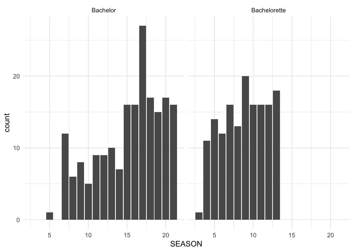
PDX Bike Counts
Follow along with these code prompts:
- Use the following code to read in data used from the annual PDX Bike Count 538:
# import bike data
untidy_bikes <- read_csv("https://raw.githubusercontent.com/apreshill/bakeoff-tidy/master/data/untidy-bike-counts.csv",
                         skip = 1,
                         na = "-") %>%
  janitor::clean_names() # optional but highly recommended
glimpse(untidy_bikes)
#> Observations: 282
#> Variables: 23
#> $ sector        <chr> "bridge", "bridge", "bridge", "city center", "ci...
#> $ site_number   <int> 2, 4, 176, 71, 72, 73, 79, 83, 84, 89, 93, 94, 1...
#> $ location      <chr> "Burnside Bridge", "Sellwood Bridge", "Morrison ...
#> $ count_time    <chr> "4-6pm", "4-6pm", "4-6pm", "7-9am", "4-6pm", "7-...
#> $ x2017         <int> 489, 180, 133, 48, 93, 65, 93, 456, 128, 80, 513...
#> $ x2016         <dbl> 478, 124, 218, 63, 112, 80, 99, 423, 135, 89, 65...
#> $ x2015         <dbl> 477, 77, 236, 62, 108, 104, 119, 629, 132, 122, ...
#> $ x2014         <dbl> 468, 133, 160, 60, 100, 68, 109, 580, 122, 451, ...
#> $ x2013         <dbl> 422, 99, 157, 57, 123, 85, 142, 535, 124, 446, 7...
#> $ x2012         <dbl> 411, 135, 172, 55, 127, 97, 83, 477, 127, 401, 6...
#> $ x2011         <int> 435, 91, NA, NA, 106, 77, 192, 441, 165, 372, 59...
#> $ x2010         <int> 373, 79, 151, 35, 133, 72, 136, 442, 130, 331, 6...
#> $ x2009         <int> 352, 96, NA, 61, 104, 72, NA, NA, 154, 258, 502,...
#> $ x2008         <int> 407, NA, NA, 72, 108, 87, NA, 392, 99, 340, 530,...
#> $ x2007         <int> 265, 97, NA, 74, 86, 52, 113, 290, 118, NA, 440,...
#> $ x2006         <int> 252, 91, 9, 36, 74, 119, 103, 191, 77, 144, 420,...
#> $ x2005         <int> NA, NA, NA, NA, NA, NA, NA, 204, NA, NA, NA, NA,...
#> $ x2004         <int> NA, NA, NA, 44, NA, NA, NA, NA, NA, NA, NA, NA, ...
#> $ x2003         <int> 138, NA, NA, NA, NA, NA, NA, NA, NA, NA, NA, NA,...
#> $ x2002         <int> NA, NA, NA, NA, NA, NA, NA, NA, NA, 191, NA, 298...
#> $ x2001         <int> 193, NA, NA, NA, NA, NA, NA, NA, NA, NA, 175, 14...
#> $ x2000         <int> NA, NA, NA, 50, 42, NA, 69, NA, 67, NA, NA, NA, ...
#> $ prior_to_2000 <int> NA, 83, 23, 39, 49, 48, 51, 163, 46, NA, 162, 24...- Gather all the bike counts for years 2000-2017 (Hint: you may need to use a
mutatewithparse_numberafter thegather). Your finished tibble should look like:
- Count bikes by sector.
#> # A tibble: 8 x 2
#>   sector           n
#>   <chr>        <dbl>
#> 1 bridge        7598
#> 2 city center  65770
#> 3 east         16618
#> 4 north        60603
#> 5 northeast    63294
#> 6 northwest    24773
#> 7 southeast   109587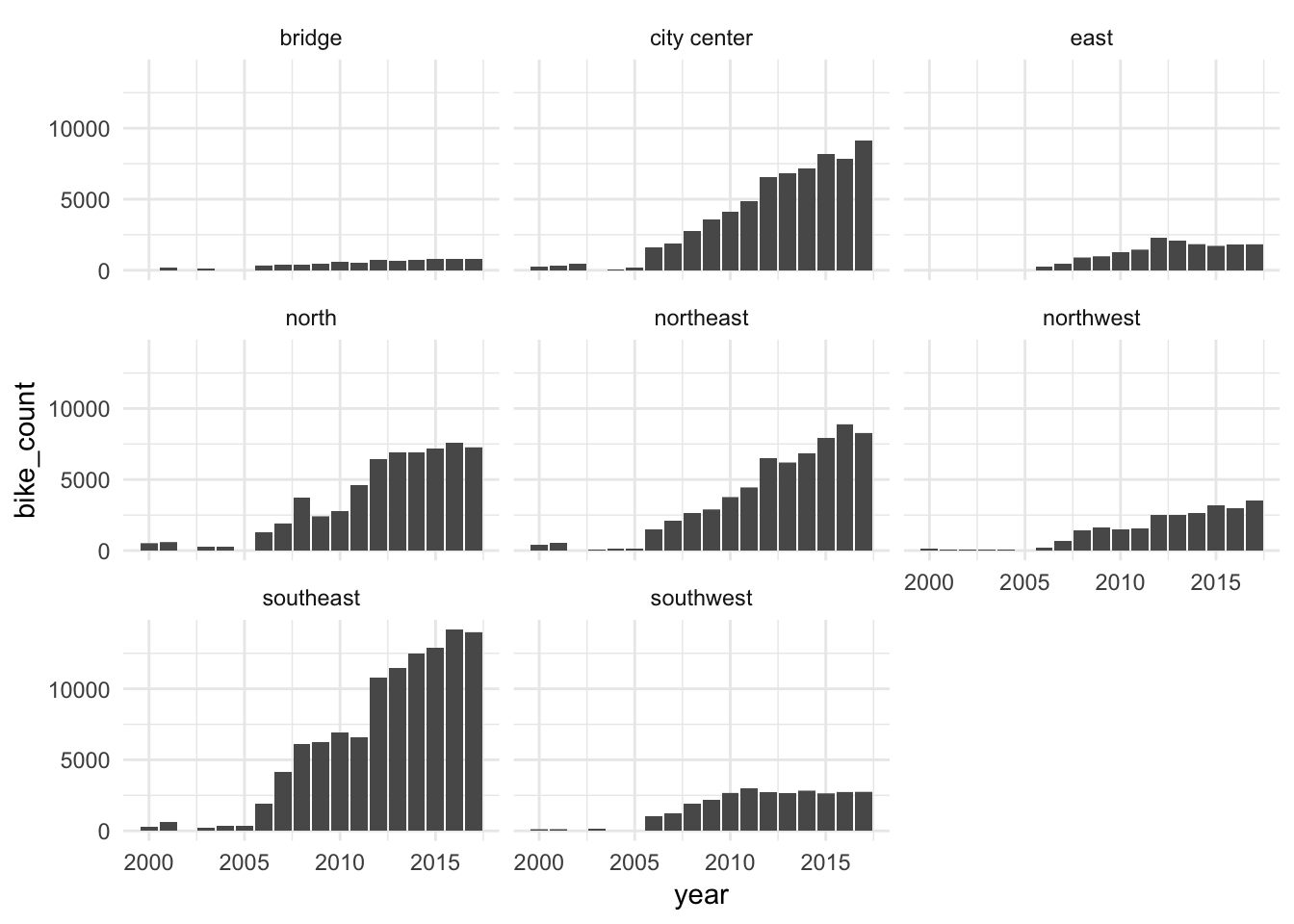
#> 8 southwest 28592- Make a plot to show the number of bikes counted across the years, facetting by sector. Has there been a steady increasing trend in bikes counted across all sectors? Which sectors have seen the most bikes counted recently?
538 Flying Etiquette Survey
Follow along with these code prompts:
- Use the following code to read in data used from 538:
# import flying etiquette data
untidy_fly <- read_csv("https://raw.githubusercontent.com/fivethirtyeight/data/master/flying-etiquette-survey/flying-etiquette.csv") %>%
  mutate_if(is.character, as.factor)
Select the participant ID and any question columns which include the word “rude”, then
gatherall the “rude” question columns.Answer some questions: how many respondents are there? how many respondents didn’t answer any of the 9 questions? Try filtering out respondents who had missing answers for all 9 questions here.
#> [1] 1040
#> # A tibble: 4 x 2
#>       n    nn
#>   <int> <int>
#> 1     2     1
#> 2     6     4
#> 3     7     1
#> 4     9   185
#> [1] 855- Summarize the data:
group_byquestion, then calculate the mean of your newrude_answercolumn to get the proportions of respondents who endorsed “yes it is rude” for each question.
#> # A tibble: 9 x 2
#>   question_asked                                                 rude_prop
#>   <chr>                                                              <dbl>
#> 1 Generally speaking, is it rude to say more than a few words t… 0.2105263
#> 2 In general, is it rude to knowingly bring unruly children on … 0.8268551
#> 3 In general, is itrude to bring a baby on a plane?              0.3027091
#> 4 Is it rude to ask someone to switch seats with you in order t… 0.2576471
#> 5 Is it rude to wake a passenger up if you are trying to go to … 0.3705882
#> 6 Is itrude to ask someone to switch seats with you in order to… 0.1705882
#> 7 Is itrude to move to an unsold seat on a plane?                0.1929825
#> 8 Is itrude to recline your seat on a plane?                     0.4121780
#> 9 Is itrude to wake a passenger up if you are trying to walk ar… 0.7341176- Make this kind of bar chart with the summarized version of your tidy data- it doesn’t need to be perfect! See below for our recreation:

For more tweaking, you can use this code to redo your labels:
abb_question <- tribble(
  ~label,
  "be chatty with seatmate",
  "knowingly bring unruly children",
  "bring a baby on a plane",
  "ask to switch seats for friends",
  "wake someone up to go to the bathroom",
  "ask to switch seats for family",
  "move to an unsold seat",
  "recline your seat",
  "wake someone up to go for a walk"
)
rude_summarized <- tidy_rude %>%
  group_by(question_asked) %>%
  summarize(rude_prop = mean(rude_answer, na.rm = TRUE)) %>%
  bind_cols(abb_question)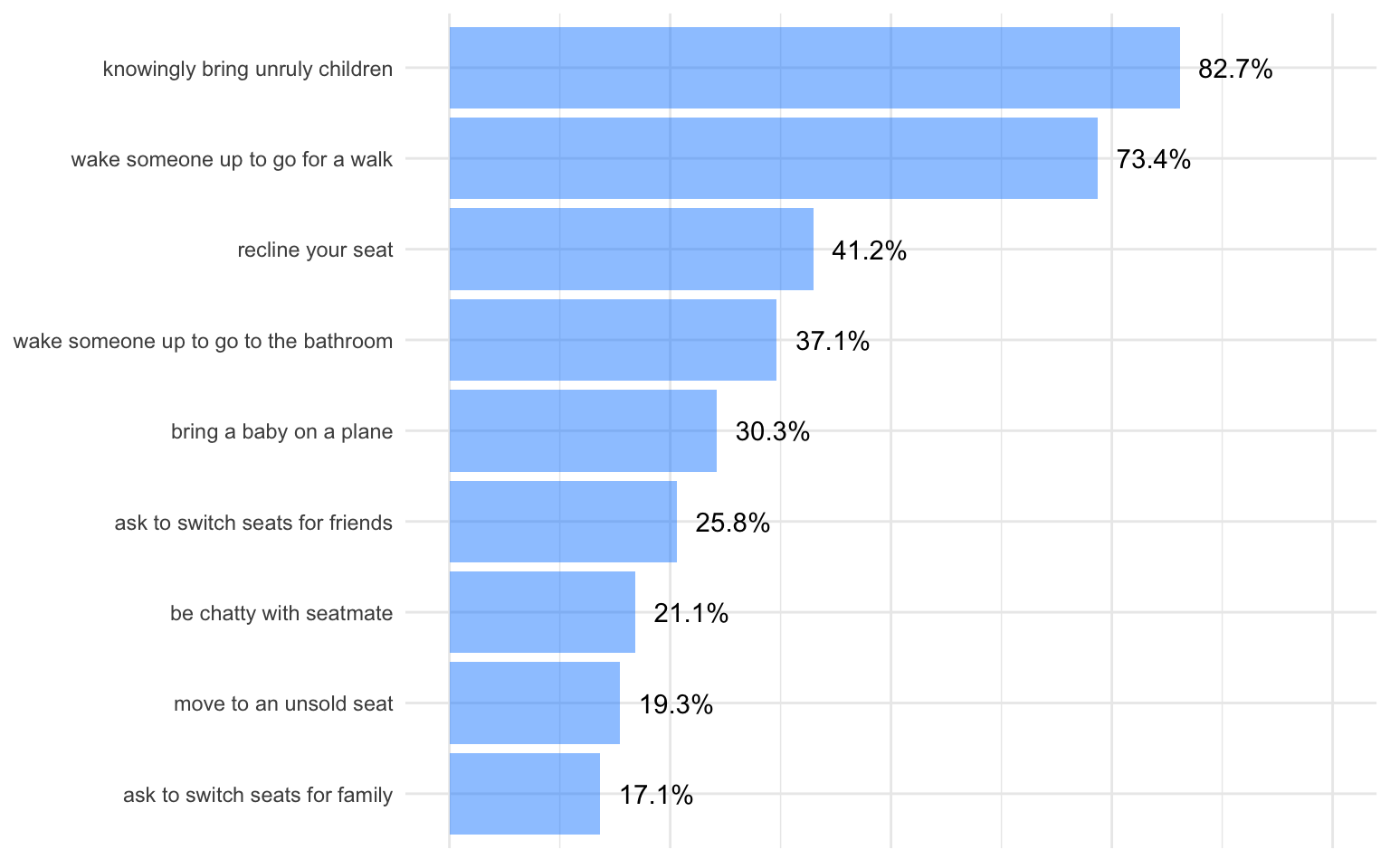
Take home message
It is untidy to have data parcelled out across different files or data frames.
It is untidy to have a conceptual variable, e.g. “word count”, “bake count”, “bike count”, “rose count”, spread across multiple variables, such as bike counts for each year. We used the gather() function from the tidyr package to stack up all these counts into a single variable, create a new variable to convey the categorical or factor variable that was previously “hidden” to us in the column names, and do the replication needed for the other variables.
Many data analytic projects will benefit from a script that marshals data from different files, tidies the data, and writes a clean result to file for further analysis.
Watch out for how untidy data seduces you into working with it more than you should:
- Data optimized for consumption by human eyeballs is attractive, so it’s hard to remember it’s suboptimal for computation. How can something that looks so pretty be so wrong?
- Tidy data often has lots of repetition, which triggers hand-wringing about efficiency and aesthetics. Until you can document a performance problem, keep calm and tidy on.
- Tidying operations are unfamiliar to many of us and we avoid them, subconsciously preferring to faff around with other workarounds that are more familiar.
Where to next?
In the next lesson 03-spread I show you how to untidy data, using spread() from the tidyr package. This might be useful at the end of an analysis, for preparing figures or tables.
Resources
- Tidy data chapter in R for Data Science, by Garrett Grolemund and Hadley Wickham
- Bad Data Handbook by By Q. Ethan McCallum, published by O’Reilly.
- Chapter 3: Data Intended for Human Consumption, Not Machine Consumption by Paul Murrell.
- Nine simple ways to make it easier to (re)use your data by EP White, E Baldridge, ZT Brym, KJ Locey, DJ McGlinn, SR Supp. Ideas in Ecology and Evolution 6(2): 1–10, 2013. doi: 10.4033/iee.2013.6b.6.f https://ojs.library.queensu.ca/index.php/IEE/article/view/4608
- See the section “Use standard table formats”
- Tidy data by Hadley Wickham. Journal of Statistical Software. Vol. 59, Issue 10, Sep 2014. http://www.jstatsoft.org/v59/i10